TL;DR
- Analyzes footfall near the British Museum using Google Maps “Popular Times”.
- Flow: collect nearby businesses, extract hourly popularity, average by hour, visualize with heatmaps.
- Stack: Python (
requests,pandas),seaborn/matplotlib; sample code + images included. - Categories covered: restaurants, cafés, galleries, pubs, theatres (cafés peak at lunch).
- Powered by Scrapingdog’s Google Maps API.
Google Maps is a great storehouse of information for businesses looking to extract phone numbers for lead generation, customer reviews for sentimental analysis, images for real-estate mapping, and footfall for analyzing the peak hours of certain places at a particular time.
In this article, we will scrape and analyze Google Maps’ Popular Times data for businesses in London during peak hours and visualize it using graphs and heat maps.
Process
In our first step, we would be scraping the list of businesses from Google Maps in a particular area of interest.
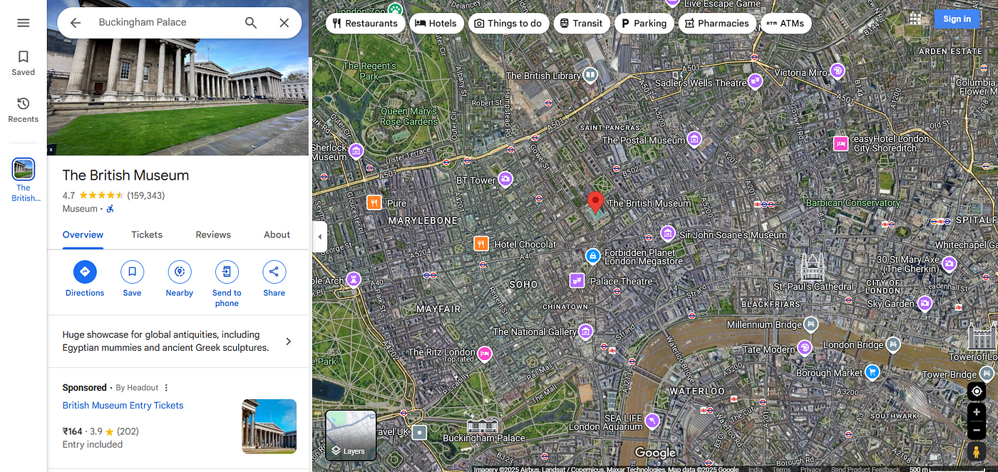
The area around the British Museum looks good for exploring the businesses of London. Here is the list of companies we are going to analyze:
- Restaurants — Indian Restaurants, French Bistros
- Cafés
- Art Galleries and Museums
- Pubs and Bars
- Theatres and Entertainment Venues
We will get the search listings for the above businesses by using our Google Maps API.
You can refer to this documentation for more information on using Scrapingdog Google Maps API.
I am sharing a sample code of how I collected the businesses for each type.
					import requests
import json
import seaborn as sns
import matplotlib.pyplot as plt
import pandas as pd

API_KEY = "APIKEY"
BASE_URL = "https://api.scrapingdog.com/google_maps"
PLACES_URL = "https://api.scrapingdog.com/google_maps/places"

# Fetch business data
def get_data():
    response = requests.get(f"{BASE_URL}?ll=@51.5181901,-0.1525433,5z&query=Indian Restaurants Near The British Museum&api_key={API_KEY}")
    data = response.json()
    businesses = []

    for place in data.get("search_results", []):
        title = place.get("title")
        place_id = place.get("place_id")

        if not title or not place_id:
            continue

        try:
            place_response = requests.get(f"{PLACES_URL}?place_id={place_id}&api_key={API_KEY}")
            place_data = place_response.json()
            popularity_scores = place_data.get("place_results", {}).get("popular_times", {}).get("graph_results", {})
        except Exception as e:
            print(f"Error fetching details for {title}: {e}")
            popularity_scores = {}

        businesses.append({
            "title": title,
            "place_id": place_id,
            "popularity_scores": popularity_scores
        })

    # Save data to JSON
    with open("businessLists.json", "w") as f:
        json.dump(businesses, f, indent=2)
    print("File written successfully!")

    return businesses
Step by Step Process
Importing Required Libraries
requests→ Used to make HTTP requests to the API.json→ Handles JSON data (parsing & saving).seaborn&matplotlib.pyplot→ Used for visualization (not used in this function but likely needed for later).pandas→ Used for data analysis (not used in this function but likely needed for later).
Setting API Constants
					API_KEY = "APIKEY"
BASE_URL = "https://api.scrapingdog.com/google_maps"
PLACES_URL = "https://api.scrapingdog.com/google_maps/places"
API_KEY→ Placeholder for the API key (should be replaced with a real key).BASE_URL→ Endpoint for Google Maps search results.PLACES_URL→ Endpoint for fetching details of a specific place.
Making an API Request for Nearby Restaurants and Extracting the Search Results
					response = requests.get(f"{BASE_URL}?ll=@51.5181901,-0.1525433,5z&query=Indian Restaurants Near The British Museum&api_key={API_KEY}")
data = response.json()

businesses = []
for place in data.get("search_results", []):
    title = place.get("title")
    place_id = place.get("place_id")
- Sends a GET request to
BASE_URL. - Initializes an empty list
businessesto store extracted data. - Loops through the search results (list of restaurants) and extracts
title(name of the restaurant) andplace_id(unique identifier for each restaurant).
Fetching Details for Each Restaurant
					try:
    place_response = requests.get(f"{PLACES_URL}?place_id={place_id}&api_key={API_KEY}")
    place_data = place_response.json()
    popularity_scores = place_data.get("place_results", {}).get("popular_times", {}).get("graph_results", {})
except Exception as e:
    print(f"Error fetching details for {title}: {e}")
    popularity_scores = {}
- Sends a second request to
PLACES_URLusing the extractedplace_idto fetch detailed information about the restaurant. - Extracts popularity data (
graph_results) from the response. - Handles errors → If the request fails, prints an error message and assigns an empty dictionary
{}topopularity_scores.
Finally, we fetched the details for each business in the businesses array and saved the data into a JSON file.
You might be thinking what is popularity_scores stored here? If you check out the Google Maps Places API at Scrapingdog, you will find the below response for each API call on a business. This is none other than popular times for a business on different weekdays.
					"popular_times": {
            "graph_results": {
                "sunday": [
                    {
                        "time": "6 AM",
                        "info": "",
                        "busyness_score": 0
                    },
                    {
                        "time": "7 AM",
                        "info": "Usually not busy",
                        "busyness_score": 7
                    },
                    {
                        "time": "8 AM",
                        "info": "Usually not busy",
                        "busyness_score": 18
                    },
                    {
                        "time": "9 AM",
                        "info": "Usually not too busy",
                        "busyness_score": 37
                    },
                    {
                        "time": "10 AM",
                        "info": "Usually not too busy",
                        "busyness_score": 39
                    },
                    {
                        "time": "11 AM",
                        "info": "Usually not too busy",
                        "busyness_score": 37
                    },
                    {
                        "time": "12 PM",
                        "info": "Usually not too busy",
                        "busyness_score": 27
                    },
                    {
                        "time": "1 PM",
                        "info": "Usually not too busy",
                        "busyness_score": 30
                    },
                    {
                        "time": "2 PM",
                        "info": "Usually not too busy",
                        "busyness_score": 48
                    },
                    {
                        "time": "3 PM",
                        "info": "Usually a little busy",
                        "busyness_score": 51
                    },
                    {
                        "time": "4 PM",
                        "info": "Usually not too busy",
                        "busyness_score": 43
                    },
                    {
                        "time": "5 PM",
                        "info": "",
                        "busyness_score": 0
                    },
                    {
                        "time": "6 PM",
                        "info": "",
                        "busyness_score": 0
                    },
                    {
                        "time": "7 PM",
                        "info": "",
                        "busyness_score": 0
                    },
                    {
                        "time": "8 PM",
                        "info": "",
                        "busyness_score": 0
                    },
                    {
                        "time": "9 PM",
                        "info": "",
                        "busyness_score": 0
                    },
                    {
                        "time": "10 PM",
                        "info": "",
                        "busyness_score": 0
                    },
                    {
                        "time": "11 PM",
                        "info": "",
                        "busyness_score": 0
                    }
                ],
             ....
            }
          }
Next, we will call this function and run our pipeline.
					businesses = get_data()
df = prepare_heatmap_data(businesses)
if not df.empty:
    generate_heatmap(df)
The prepare_heatmap_data and generate_heatmap data will help us in organizing the data for heatmap and generating the graphic respectively.
					def normalize_hour_string(hour):
    # Replace non-breaking spaces and standardize to the format used in 'columns'
    return hour.replace('\u202f', ' ').strip()

def prepare_heatmap_data(businesses):
    columns = ["6 AM", "7 AM", "8 AM", "9 AM", "10 AM", "11 AM", "12 PM", "1 PM", "2 PM", "3 PM", "4 PM", "5 PM", "6 PM", "7 PM", "8 PM", "9 PM", "10 PM", "11 PM", "12 AM", "1 AM", "2 AM", "3 AM", "4 AM", "5 AM"]
    heatmap_data = []

    for business in businesses:
        title = business["title"]
        daily_scores = {hour: [] for hour in columns}  # Initialize all hours with empty lists

        for day, hours in business["popularity_scores"].items():
            for hour_data in hours:
                hour_index = normalize_hour_string(hour_data['time'])
                if 'busyness_score' in hour_data:
                    daily_scores[hour_index].append(hour_data['busyness_score'])

        # Calculate the average popularity per hour across the week or fill with zero
        daily_avg = [(sum(scores) / len(scores) if scores else 0) for scores in daily_scores.values()]
        heatmap_data.append({"business": title, **dict(zip(columns, daily_avg))})

    return pd.DataFrame(heatmap_data)
Step-by-step explanation
- Normalize Hour Strings: Replaces non-breaking spaces (
\u202f) in hour strings.
Prepare Heatmap Data:
- Defines hourly time slots (6 AM — 5 AM the next day).
- Initializes
heatmap_datalist to store processed business popularity scores. - Loops through each business.
- Initializes an empty list for each hour to store multiple days’ data.
- Iterates through popularity scores and appends busyness values for each hour.
- Computes average busyness per hour.
- Converts the result into a Pandas DataFrame.
Finally, we generate the heatmap.
					# Generate heatmap
def generate_heatmap(df):
    plt.rcParams['font.sans-serif'] = ['Arial Unicode MS']  # for unicode characters
    plt.rcParams['axes.unicode_minus'] = False  # for minus sign characters
    columns = ["6 AM", "7 AM", "8 AM", "9 AM", "10 AM", "11 AM", "12 PM", "1 PM", "2 PM", "3 PM", "4 PM", "5 PM", "6 PM", "7 PM", "8 PM", "9 PM", "10 PM", "11 PM", "12 AM", "1 AM", "2 AM", "3 AM", "4 AM", "5 AM"]
    heat_data = df.set_index("business").reindex(columns=columns)

    plt.figure(figsize=(15, 8))
    sns.heatmap(heat_data, cmap='YlOrRd', annot=True, fmt=".0f", linewidths=.5)
    plt.title('Popularity by Hour')
    plt.xlabel('Hour of Day')
    plt.ylabel('Business')
    plt.xticks(rotation=45)
    plt.tight_layout()
    plt.savefig("heatmap.png")
    plt.show()
Step-by-step explanation:
- Sets up Matplotlib for Unicode support.
- Formats DataFrame for heatmap plotting.
- Creates the heatmap with Seaborn.
- Uses ‘YlOrRd’ color gradient (yellow-to-red).
- Annotates heatmap cells with numerical values.
- Saves the heatmap as an image (
heatmap.png).
Running this program will give you the following heatmap.
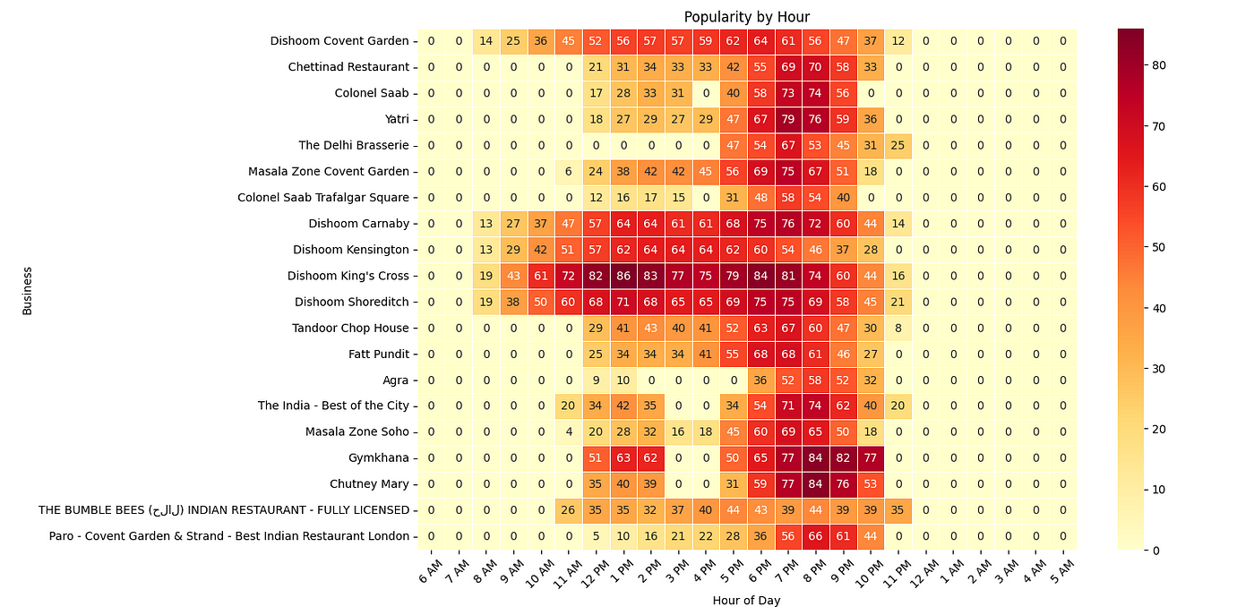
Similarly, you can run the programs for other queries also.
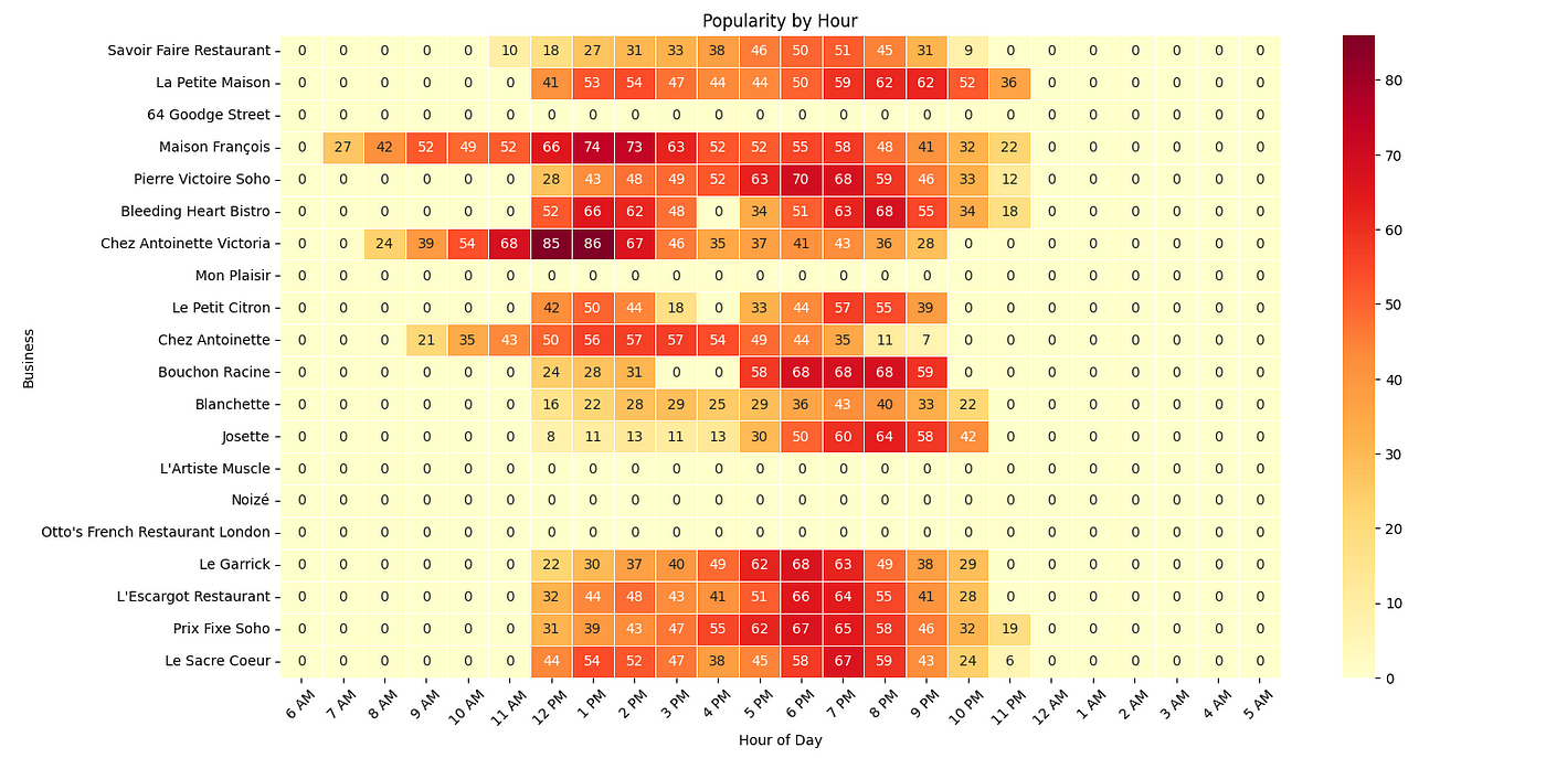
French Bistros
Cafes
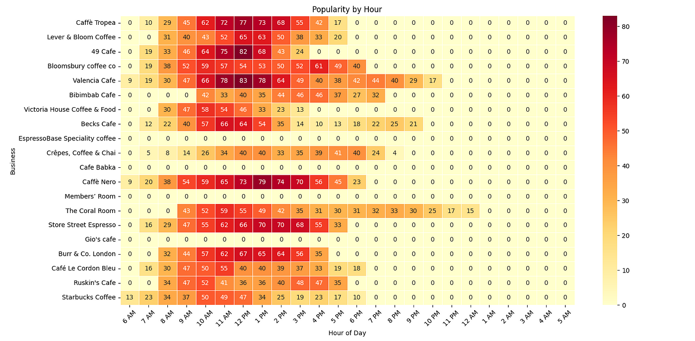
Most of these cafes peak near lunchtime.
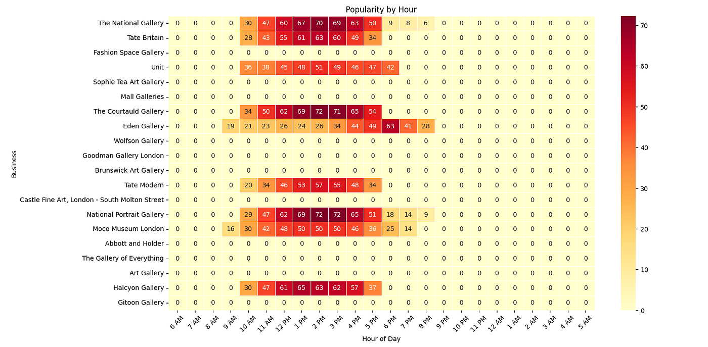
Art Galleries and Museums
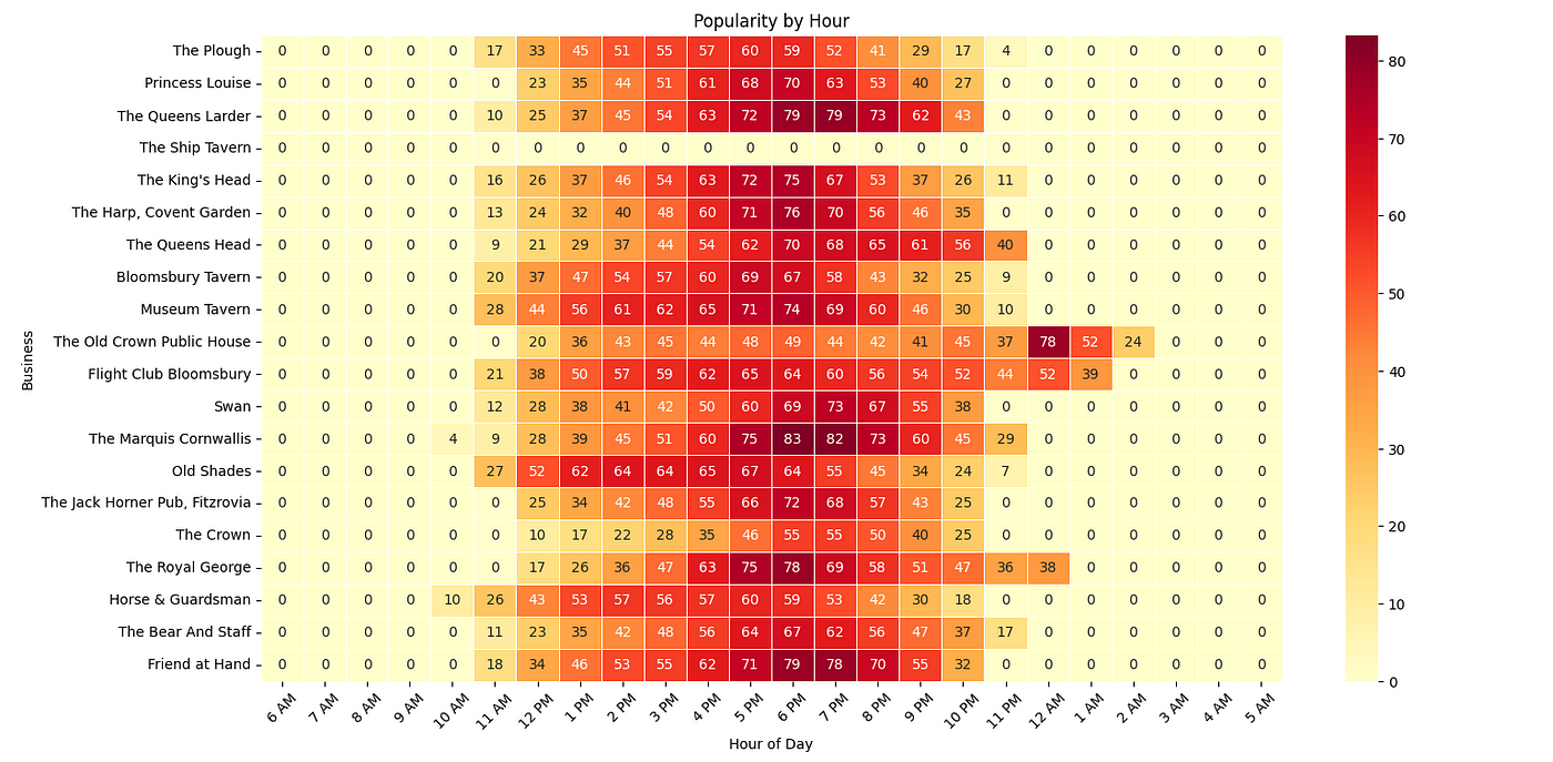
Pubs and Bars
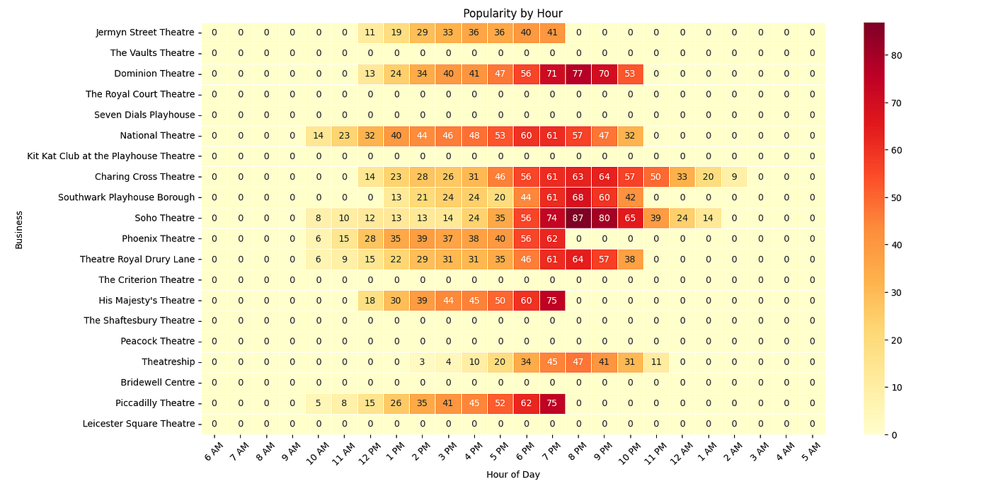
Theatres and Entertainment Venues
Conclusion
Google Maps generates interesting data on businesses that can be used for creating studies and research.
In this article, we analyzed the popular times for various businesses in London using Scrapingdog Google Maps API. I hope you found it helpful! If you did, please consider sharing it on social media.
If you want to analyze free local business data, you can use this tool, extract 20 local businesses’ data from a location.
Thanks for reading! 👋